Watching the Socceroos go out to Egypt on penalties at the 2026 World Cup made me wonder about player height vs penalty success rate. Both Australian defenders who missed – Harry Souttar and Lucas Herrington – are tall. Souttar is 198 cm. Herrington is 193 cm.
On the back of the Champions League shootout where Gabriel (190cm) also missed, I wondered if there is anything statistically meaningful relating to player height and penalty success rate.
The question
Is there a relationship between a player’s height and whether they score from the spot? And does it differ for in-game penalties versus shootouts, where the pressure is obviously different?
The data
For penalties, I used the dataset from Vollmer, Schoch and Brandes (2024) – roughly 51,000 cleaned penalty attempts from European men’s football between 2012–13 and 2022–23, plus World Cups in 2014, 2018 and 2022. Each row is a single kick: scored or not.
For height, I used Transfermarkt data, matching players by name.
Of the 51,007 penalties, the height data matched for 29,803 (about 58%). The unmatched penalties are mostly from smaller leagues where Transfermarkt coverage is thinner.
The matched sample covers 9,744 unique takers, heights ranging from 160 cm to 203 cm, with a mean of about 182 cm.
What the numbers say
Shootouts are harder
Context
Penalties
Success rate
In-game
20,827
81.4%
Shootout
8,976
75.5%
That ~6 percentage point gap matches what Vollmer et al. found. Shootouts are different.
Height? Not signficant
Here’s success rate by 10 cm height band, all players, all positions:
Height
Attempts
Success rate
160–169 cm
624
78.4%
170–179 cm
9,902
79.5%
180–189 cm
16,105
79.7%
190–199 cm
3,118
79.8%
200–209 cm
54
83.3%
From 170 cm upward, it’s essentially a flat line around 79–80%. The 200+ cm group looks better, but with only 54 attempts it’s not a large enough data set.
Using the 180 cm threshold:
In-game: under 180 cm scored 81.4% of the time; 180 cm and over scored 81.4%
Shootout: under 180 cm scored 74.9%; 180 cm and over scored 75.9%
Splitting into height quartiles tells the same story. The tallest quarter doesn’t consistently underperform the shortest.
Statistically, the correlation between height and scoring is effectively zero (Pearson r = 0.003, p = 0.57). A logistic regression gives an odds ratio of 1.001 per centimetre of height – meaning each extra centimetre changes your odds of scoring by about 0.1%. That’s not significant. The shootout interaction term is also insignificant (p = 0.95), so height doesn’t affect in-game and shootout penalties differently either.
Short (?) version: being tall doesn’t make you more likely to miss, or more likely to score.
Look at defenders only, the results are similar – no significant impact on success based on player height.
Earlier in the year I completed the Stanford University Machine Learning course at Coursera. It was created by Prof Andrew Ng and was a fascinating and enjoyable course. There was more mathematics involved than I had anticipated but pace of the lectures and assignments made it an enjoyable challenge to complete. I highly recommend this course for anyone interested in learning more about different machine learning algorithms and how to apply these to real world problems.
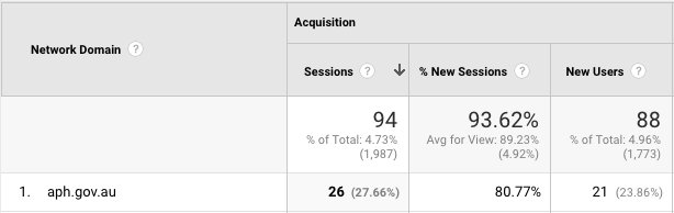
In the month after my “Analysis of MP’s vocabularies using Hansard” post, I had more traffic than usual from Canberra. Interestingly, Google Analytics shows that the largest group of these (26) came from the aph.gov.au Network Domain, which is Parliament House.
As a way to get some more experience with various data analysis tools I needed an engaging side-project. Politics interests me, so an analysis of the publicly available Hansard transcripts from Parliament seemed like a good project.
By analysing the contents of MPs’ speeches in Parliament, I hoped to be able to get a sense of the breadth of their vocabularies (however accurate or inaccurate this might be), and see how they compare with their colleagues. By determining the total number of unique words spoken compared with the total number of words spoken for each Member, it is possible to make comparisons between the “functional” vocabularies of all MPs.
Intelligence and the size of a person’s vocabulary have long been considered analogous, however perhaps a large vocabulary merely indicates a capability or potential for sophisticated thought, rather than a direct indication of this.
There are plenty of caveats with this type of analysis, and some of the reasons why these results might not be an accurate representation of a Member’s true vocabulary are as follows:
They could be intentionally staying “on message”
They could be keeping their language simple to be more readily understood
The transcripts used in this project are from both the House of Representatives and Senate, from the 7th of February 2017 to the 17th of August 2017. There are 75 different transcripts, 227 Members which translated into 15.3 million words in the database. To extract only words from the transcripts, all URLs, numbers and punctuation have been removed. Word “uniqueness” is determined after a lowercase transformation, i.e. a reference to “Cash” (as in Michaelia) would be considered a match with “cash” (as in $).
It is also worth noting that verb conjugation is essentially ignored. I.e. “runs”, “running” and “ran” would be considered as 3 unique words, when in a practical sense they are the same verb.
Regardless of these potential factors, the results are interesting and presented here as is.
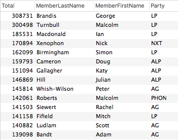
The total overall word count by Member gives us this:
Note that Brandis doesn’t necessarily have the biggest vocabulary, he has only spoken the most words in Parliament during this period.
Uniqueness by total words spoken
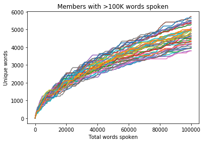
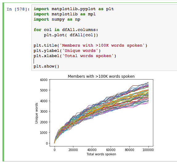
Using 100,000 spoken words as the threshold for inclusion, out of the 227 Members there are 42 from both the House of Representatives and Senate who have reached this number. If we graph the progression of the total unique word count by the total word count, we get a relatively even distribution (colours are random).
Party Colours
If we chart these same 42 Members on a bar graph using their Party colour as the bar colour a few things become apparent:
Interestingly, at the 100K mark Malcom Roberts has the most unique words, just in front of Scott Ludlam
The Greens are over-represented at the top – 40% of the top 5 places
The Labor Party mean appears to be above average
The bottom of the table is relatively heavy with Liberal Party conservatives
(Notes on the colours: all parties are their official colour apart from Australian Conservatives who are pink (sorry Bernadi), Independents who are grey and Nationals who are black, as green and yellow are both already taken)
Party by Party
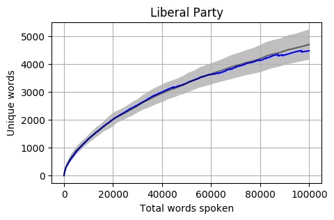
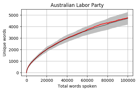
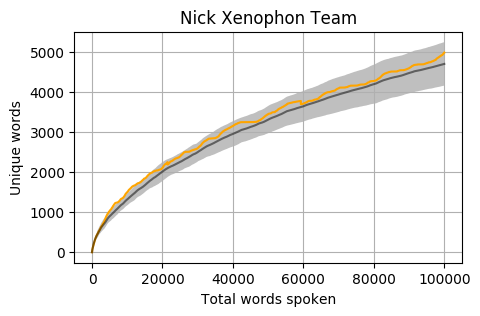
Looking at the mean for each party we get the following. Note that the mean is calculated word by word and each Member’s total word count is different. When one Member is no longer part of the calculation, the overall mean can jump a little (as seen in the Liberal Party and Greens graphs).
The grey bar represents the mean for the 42 Members who reached 100,000 words. The grey area around the bar is one standard deviation from the mean.
Head to head by Portfolio
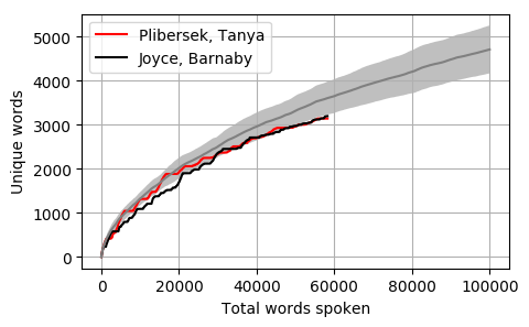
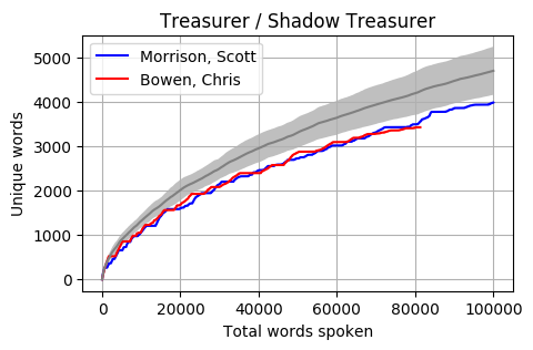
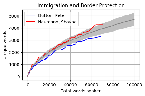
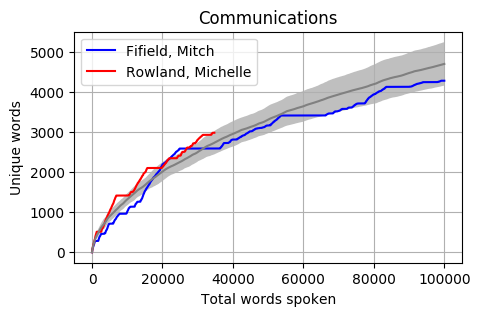
Looking at Members individually gives some interesting results. Some of these Members haven’t reached the 100k mark yet however the trajectory is relatively obvious. The following graphs pit the Minister and Shadow Minister against each other for a few of the different portfolios and positions. Until I can explore the difference between speeches and answers, the impact of speechwriters on these results is unknown.
The Cabinet
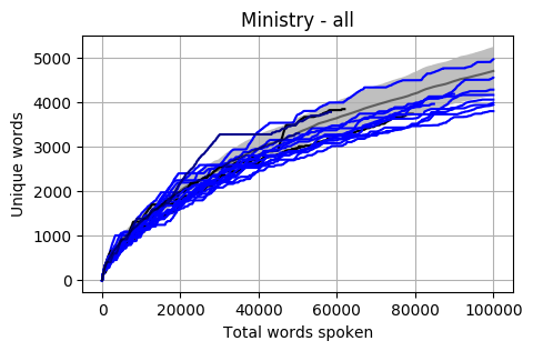
Looking at a graph of the complete Members of Cabinet the results are a little concerning. Most are below the Mean and a good proportion are also below one standard deviation.
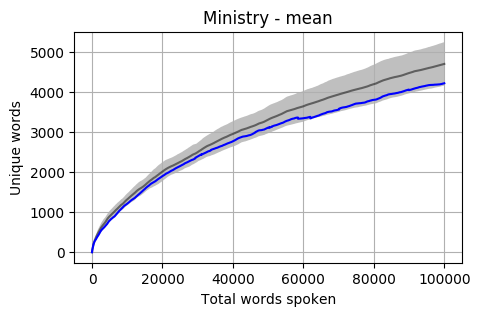
The mean of all Cabinet Members is below, and it is sitting almost at one standard deviation below the overall mean.
Up Next
There are a few other dimensions that I plan to explore in the coming weeks:
Speech context
The data is ready to segment by Speeches, Questions and Answers, and I believe that we might find some interesting differences between prepared speeches and answers that could indicate a good/bad speech writer.
Overall uniqueness
At the moment uniqueness is being judged member by member. Exploring who has the most unique words across all members (and what these are) could also be interesting.
Self reference
Could some analysis showing who refers to themselves the most (“I”, “me”, “myself”, “my”, etc) show us who is the most self-important?
Historical comparison
This data has only been for 2017. How would previous governments or cabinets compare with today?
UK Parliament
Are UK Hansard archives available in XML format?
Footnotes
This is a personal side-project unrelated to my work or employer. The accuracy of the results is not guaranteed and I could have made some fundamental errors in the code. If you have any questions, concerns, suggestions or requests please leave me a comment below.
Some technical details about the process for the Hansard data analysis project:
Downloading Hansard transcripts (XML) from the Parliament of Australia website using a Python script (some Javascript hackery was required to get the proper path)
Python with BeautifulSoup to parse the XML and write individual words to a local database, with a reference to the Member along with the context of the word (session, time, speech, question, answer, etc)
Stripping out punctuation, numbers, apostrophe + ‘s’, URLs, etc.







Recent Comments